Monte Carlo Prediction & Temporal Difference

In this article, we consider learning methods for estimating value functions and discovering optimal policies. Unlike the previous article, here we do not assume complete knowledge of the environment.
in a model-Free algorithm, it’s used if we don’t know the dynamic and/or rewards model.

if we know the model P(s ′|s, a) rewards and Expectation over next states computed exactly,Dynamic programming compute this by Bootstrapping the rest of the expected return by the value estimate Vₖ₋₁.

Monte Carlo & TD methods require only experience sample sequences of states, actions, and rewards from actual or simulated interaction with an environment. Learning from actual experience is striking because it requires no prior knowledge of the environment’s dynamics, yet can still attain
optimal behavior. Learning from simulated experience is also powerful. Although a model is required, the model need only generate sample transitions, not the complete probability distributions of all possible transitions that is required for dynamic programming (DP). In surprisingly many cases it is easy to generate experience sampled according to the desired probability distributions, but infeasible to obtain the distributions in explicit form. first we will toke about Monte Carlo (MC) and then Temporal Difference (TD).

Monte Carlo

Monte Carlo methods are ways of solving the reinforcement learning problem based on averaging sample returns, it’s a very wide used algorithm, and a lot of programs use it like AlphaGo which we will try to implement in the future.

Gₜ= Rₜ+ γRₜ₊₁+ γ²Rₜ₊₁+ · · · (1)

V(s) = E ₜ∼π [Gₜ|sₜ= s] · · · (2)

The value function is the expectation over trajectories T generated by following π.in another world its just the mean return

To ensure that well-defined returns are available, here we define Monte Carlo methods only for episodic tasks. That is, we assume experience is divided into episodes, and that all episodes eventually terminate no matter what actions are selected. Only on the completion of an episode the value estimates and policies changed. Monte Carlo methods can thus be incremental in an episode-by-episode sense, but not in a step-by-step (online) sense.The term Monte Carlo is often used more broadly for any estimation method whose operation involves a significant random component. Here we use it specifically for methods based on averaging complete returns (as opposed to methods that learn from partial returns like TD).

Note : as we say before MC is a Free-model algorithm, it does not require a Dynamic model and also does not assume the state is a Markovian state, in another world the estimates for each state are independent. The estimate for one state does not build upon the estimate of any other state, as is the case in DP. In other words, Monte Carlo methods do not bootstrap.

There are two approaches for the Monte Carlo algorithm First-visit and Every-visit there is a little difference between these two approaches, we will explain well in a later article but for now, we can say the First-visit estimator is unbiased while Every-visit is bias estimator

we will first introduce the Evaluation algorithm which evaluates some policy π then we will introduce
the control algorithm which improves the policy to make better action.

First Visit Monte Carlo Evaluation.

by while True we mean loop as possible as can. for the second loop, we use the reverse time step, and for computing the discount return by doing that we save a lot of computation. for example lets say I have episode with 3 time step and the rewards is as follows [5, −2, 8] if I want to compute the return for first time step and lets say γ is 0.6. then.

G₀ = 5 + 0.6 ∗ −2 + 0.6²∗8 = 6.68
G₁ = −2 + 0.6 ∗ 8 = 2.8
G₂ = 8

hear we need to compute the return for each state from beginning, the reverse technique compute them all in one shot or in incremental technique.

G₂ = 8
G₁ = −2 + 0.6 ∗ G₂ = 2.8
G₀ = 5 + 0.6 ∗ G₁= 6.68

if we want to use Every-visit we just omit the if line from the previous algorithm now we will improve this algorithm for the control problem as we say before, I don’t want to just evaluate the policy I want to learn policy to make a decision. as before but now we will use the Q function which
is the expected return when starting in state s, taking action a, and thereafter following policy.

First Visit Monte Carlo for control.

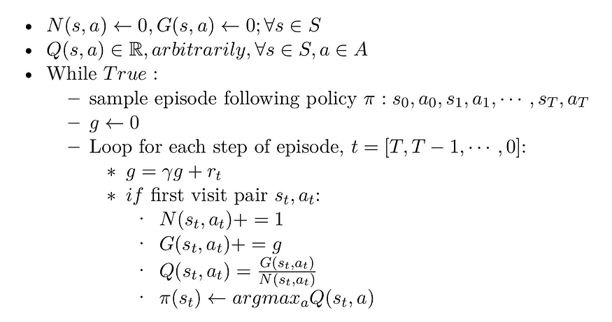
there are two issues in this implementation:

1. is inefficient because, for each state-action pair, it maintains a list of all returns and repeatedly calculates their mean. It would be more efficient
   if we use increment techniques.
2. many state–action pairs may never be visited

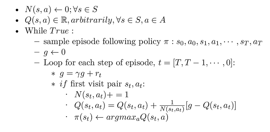
for the first problem, we can use the incremental technique so we don’t need to keep track of all state-action pairs which may take a lot of memory. for the other problem we should use an exploration algorithm
(UCB, ϵ−greedy, …), this is a very important topic which we will try to write an article about later, but for now, I am going to explain shortly ϵ−greedy algorithm which we will use a lot when we will implement Algorithms in the future.

ϵ−greedy Algorithm

for free-model algorithm can work only if the exploration policy explores the world thoroughly enough. Although a purely random policy is guaranteed to eventually visit every state and every transition many times, it may take an extremely long time to do so. Therefore, a better option is to use the ϵ-greedy policy (ϵ is epsilon): at each step it acts randomly with probability ϵ, or greedily with probability 1–ϵ . The advantage of the ϵ-greedy policy (compared to a completely random policy) is that it will spend more and more time exploring the interesting parts of the environment, as the estimator get better and better, while still spending some time visiting unknown regions of the environment. It is quite common to start with a high value for ϵ(e.g., 1.0) and then gradually reduce it (e.g., down to 0.05). The pseudocode:

• ϵ ← 1
• a ← random − value ∈ [0, 1]:
• if a < ϵ: take random a ∈ A.
• else: chose the greedy action using the estimator (e.g. argmax a Q(s, a))
• ϵ ← update

First Visit Monte Carlo using Increment technique.

Temporal-Difference

If one had to identify one idea as central and novel to reinforcement learning, it would undoubtedly be temporal-difference (TD) learning. TD learning is a combination of Monte Carlo ideas and dynamic programming (DP) ideas. Like Monte Carlo methods, TD methods can learn directly
from raw experience without a model of the environment’s dynamics. Like DP, TD methods update estimates based in part on other learned estimates, without waiting for a final outcome (they bootstrap).

TD learning as before its model-free algorithm, I don’t need the Dynamic model to learn the policy. There is an Advantages over MC, wherein MC I need to wait until the end of the episode to make an update, and that makes the learning processes slow. while in TD it’s online training I made an
update after each transition if I am using TD(0) or after λ transition if I am using T D(λ) where λ refer to the steps to be made in the future. another advantage is we can use TD in continuing tasks and have no episode at all.

for MC algorithm

V(sₜ) ← V(sₜ) + α[Gₜ− V(sₜ)]…… (3)

in the above equation the Gₜ is the full return for state s at time step t while for TD(0) update is as follow.

V(sₜ) ← V(sₜ) + α[Rₜ+γV(sₜ₊₁)− V(sₜ)]…… (4)

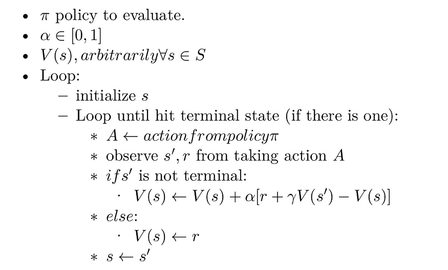
where α is the step size (learning rate) and γ discount factor. so we sampling from world a tuple (sₜ, aₜ, rₜ, sₜ₊₁) then do update following (4).

The TD target is : Target = Rₜ+ γV(sₜ₊₁)

the TD error is : δₜ= Rₜ+ γV (sₜ₊₁) − V (sₜ)

the TD error is the difference between the current estimate value and the next estimate value, in another world how much I am far away from the expectation of the next state. TD error is not necessarily going to zero.

TD(0) Evaluation

before we move on we will briefly talk about off/on-policy. for on-policy we learn to estimate and evaluate a policy, from experience obtained from following that policy . while in off-policy learn to estimate and evaluate policy using experience gathered from following different policies.

TD control

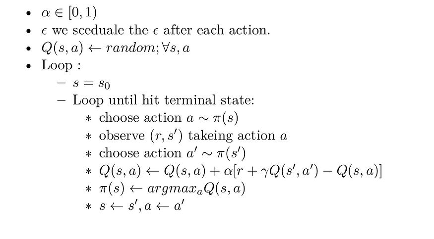
We turn now to the use of TD prediction methods for the control problem. we will talk about two algorithms SARSA and Q-learning. sarsa is abbreviation for state,action,reward,next_state,next_action. and its

SARSA on-policy TD control.

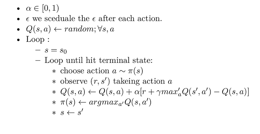
Q_learning off-policy TD control.

In this case, the learned action-value function, Q, directly approximates Q*, the optimal action-value function, independent of the policy being followed

summary

in this article we introduce Monte Carlo algorithm and Temporal Difference algorithms which they are make up the of the RL. you should read this article very well and understand all details because in the next article we will start the code using the algorithms in this article.

I hope you find this article useful and I am very sorry If there is any error or Misspelled in the article, Please do not hesitate to contact me, or drop comment to correct things.

Khalil Hennara
Ai Engineer at MISRAJ