Markov Decision Processes & model Base Algorithm

In the early 20th century, the mathematician Andrey Markov studied stochastic processes with no memory, called Markov chains.
Such a process has a fixed number of states (finite), and it randomly evolves from one state to another at each step.

The probability
for it to evolve from a state s to a state s’ is fixed, and it depends only on the pair (s, s’), not on past states (this is why we say that the system has no memory)

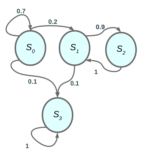
Example of markove chain.

The Markov property say that The current state is sufficient to represent the whole history of the world.

P (sₜ₊₁ |sₜ, aₜ) = P (sₜ₊₁ |hₜ) … (1)

in equation (1) hₜ represent the full history from first step until current time step. as we say earlier that the transition from one state to other its depend only on the current state, in other world the current state represent full history.

Example:
auto-drive car, the current state is sufficient for the agent to know what action to fire.
unthinking about how much the current state is sophisticated the neighbor car, pedestrian, light, engine, etc …
but if I represent all this feature in one vector represent the current state then this vector (state) its sufficient to take action.

Markov Processes

as in Figure.1 the MP is sequence of states with markove property. The full definition .

1. S finite set of states
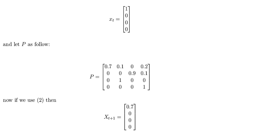
2. P is dynamic model of the world P (s ₜ = s ′ |sₜ= s) lets call the vector X ₜ is the state representation at time step t and The matrix P is the dynamic model with NxN dimension N is number of states

X ₜ₊₁ = P ∗ Xₜ … (2)

where ∗ is dot-product

Example: the states space have 4 state and we represent each state as one-hot vector as in Figure.1

Markov Reward Processes

in MRP we make a little twist we add Reward function to Markov Chain
we still have dynamic model as before but with reward function.
Definition of MRP:

1. S is finite set of states (s ∈ S)
2. P is Dynamic model that specifies P(s ₜ₊₁ = s|s ₜ= s ′ )
3. R is the Reward function R(sₜ= s) = E[rₜ |sₜ = s]
4. γ is discount factor γ ∈ [0, 1]

the reward function if you are in a particular state what is the expected reward get from that state. and the discount factor γ allows us to think about how much we weigh immediate rewards vs feature rewards.
now after we add the reward to the world we can define Return and The Expected Return as before we define the return as follows.

Gₜ= Rₜ+ γRₜ₊₁ + γ²Rₜ₊₂ + · · · (3)

V = E[Gₜ|sₜ= s] = E[rₜ+ γrₜ₊₁+ γ²rₜ₊₂ + · · · |sₜ= s] … (4)

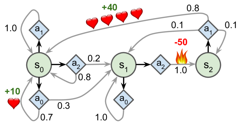
in Figure 2 we can see a Markov Processes with rewards in each state and the transition on the arch.

Note :

1. if the processes is deterministic then G t and V are same, but if the processes is stochastic they will be different
2. if episode length are always finite,you can use γ = 1

Computing The Value of MRP.

1. could estimate by simulation: Generate a large number of episodes, Average return, compute the Expected return.
2. if the world is Markovian then we can decompose the Value function in
   V (s) = R(s) + γ ∑ P (s ′ |s) V (s ′ ) … (5)

if we are in finite stetes MRP we can write V (s) using Matrix notation.

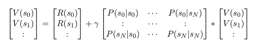
V = R + γP V … (6)

where V and R vector with N elements and P is matrix with NxN shape.
we can solve (6) using linear Algebra.

V − γP V = R
V (I − γP ) = R
V = (I − γP )⁻¹R

to solve this equation we need O(N³) operation to compute the inverse of the matrix, if N is big then it’s infeasible. fortunately, we can solve the problem using the iterative algorithm.

3. Iterative algorithm using Dynamic Programing
a. initialize V (s) = 0 for all s.
b. for k = 1 until convergence:
for all s ∈ S:
Vₖ(s) = R(s) + γ ∑ ₛ ′ P (s ′ |s)Vₖ₋₁ (s ′ )

the computational complexity is O(N²) where N is The number of states.

Markov decision processes

were first described in the 1950s by Richard Bellman. They resemble Markov chains but with a twist: at each step, an agent can choose one of several possible actions, and the transition
probabilities depend on the chosen action. Moreover, some state transitions return some reward (positive or negative), and the agent’s goal is to find a policy that will maximize reward over time.
its just MRP + actions
Definition of MDP.

1. S is finite set of states (s ∈ S)
2. A is set of actions a ∈ A
3. P is Dynamic model for each action that specifies P(sₜ₊₁ = s|sₜ = s ′ , aₜ=a)
4. R is the Reward function R(sₜ= s, aₜ= a) = E[rₜ|sₜ= s, aₜ= a]
5. γ is discount factor γ ∈ [0, 1]

MDP is a tuple (S, A, P, R, γ)

as we say in the previous article, the policy specifies what action to take in each state. π(a|s) = P (aₜ= a|sₜ= s)
if we add a policy to MDP we back to MRP and this is a very important property because now we can use the calculation technique for MRP with MDP if we are using some policy. this is true because you specify your distribution over action.

Rπ (s) =∑ₐ π(a|s)R(s, a)

Pπ (s′ |s) = ∑ₐ π(a|s)P (s ′ |s, a)

policy evaluation algorithm

1. initialize V (s) = 0 for all s.
   2. While True:
   for all s ∈ S:
   V ₖ(s) = R(s, π(s)) + γ ∑ₛ ′ π (s ′ ) P (s ′ |s, π(s))Vₖ₋₁
   |Vᵢ− Vᵢ₊₁ | < ϵ break

This is a bellman Backup for a particular policy.

Control

we don’t want just evaluate the policy we want to learn a good policy and the is the Control to
compute the optimal policy:

π*= argmax_π V … (7)

in the equation above we take the maximum overall policies that make the value function as max as possible. one option is searching to compute the optimal policy the number of deterministic policies is |A|ˢ where |A| is the number of actions and |S| is the number of states.

Policy iteration is generally more efficient.

Policy Iteration Algorithm
1. policy Iteration algorithm using Dynamic Programing
1. set i=0
2. initialize π 0 (s) randomly for all s.
3. While True:
Vπᵢ= policy evaluation on πᵢ
πᵢ₊₁ = policy improvment
i + = 1
|πᵢ− πᵢ₊₁ | < ϵ break.

we already see the policy evaluation algorithm but what about policy improvement before we write the pseudocode of policy improvement we will introduce a very important function called state-action function. this function compute the value of each state s taking action a so we compute the value for each pair (s, a)

Q π (s, a) = R(s, a) + γ ∑ₛ ′ P (s ′ |s, a) Vπ (s ′ ) … (8)

policy improvement
policy improvement algorithm
1. for s ∈ S,a ∈ A:
2. Q πᵢ (s, a) = R(s, a) + γ ∑ₛ ′ P (s ′ |s, a)V πᵢ(s ′ )
3. πᵢ₊₁ = argmax ₐQπ for all s ∈ S
4. return πᵢ₊₁

so why this work.
from the policy improvement we say that πᵢ₊₁ = argmax_a Qπ for all s ∈ S what this equation means, if I take the max over action for one state then following the old policy I am sure that I make better or at least us the previous policy, if I take the max overall action for each state then I guarantee that this new policy better than previous one. the max over action is the state value
function from the defeneation.

max Q πᵢ (s, a) = R(s, a) + γ ∑ₛ ′P (s ′ |s, a)V πᵢ(s ′ ) = V πᵢ(s)

we decline that policy improvement has monotonic improvement. which mean; ∀s ∈ S; V πᵢ≤ V πᵢ+1

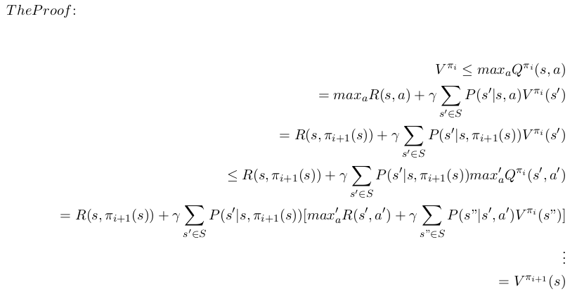
we expanded the definition until we reach the definition of V π i+1
The last thing we will toke about is the value iteration algorithm which is convergence as policy iteration but with different aspects.

Value Iteration.

let’s define the Bellman Backup Operators

BV(s) = max ₐ R(s, a) + γ ∑ₛ ′P (s ′ |s, a)V (s ′ )

BV yields a value function over all states s

Value Iteration algorithm
1. set K = 1
2. set V (s) = 0; ∀s ∈ S.
3. While True:
for s ∈ S:
Vₖ₊₁ (s) = max ₐ R(s, a) + γ ∑ₛ ′P (s ′ |s, a)Vₖ(s ′ )

|Vₖ− Vₖ₊₁ | = 0 break.

if we use the view of Bellman backup :
V ₖ₊₁ = BVₖ

the algorithm works as follows we startup and initialize $V(s) = 0 $ and then loop until we converge,
basically for each state do bellman backup. so for the first backup, we take the max immediate reward which is the best to do if we have one step to do, then we continue with backup in another world what is the best move to do if I have to take 2 steps,3 steps and so on. for example, if I am a beginner in Chess then I find The best move to take unthinking in the future scenario, but as I train and have the experience I can make a better move by simulating the next
moves that can happen on the board.

the proof of Value Iteration convergence.
Let O be an operator, and |x| norm of x, if |OX − OX ′ | ≤ |X − X ′ | then O is contraction operator. O is function in analysis thinking and Matrix in algebra, so lets say that V, V ′ is two vector and Multiply each of them with matrix O if the O is contraction operation then the distance(Norm)
between this two vector get smaller.

Theory: the bellman operator is contraction operator if γ < 1.
proof :
Let |V − V ′ | = max ₛ|V (s) − V (s ′)| is the infinity norm

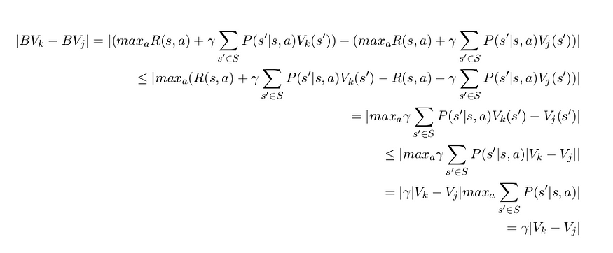
so Even if all inequalities are equalities,this is still a contraction if γ < 1.

Summary

in this article we introduce Markov decision Processes and model base Algorithm, which use to find the best action to do in some situation(state) if we know the dynamic model (The model of the world ). we introduce Policy Iteration , Value Iteration algorithm which as we proof converge to the optimal policy if I role the algorithm for enough time.in the next Article we will introduce Free-model Algorithm where I can learning value function not just planning .

I hope you find this article useful and I am very sorry If there is any error or Misspelled in the article, Please do not hesitate to contact me, or drop comment to correct things.

Khalil Hennara
Ai Engineer at MISRAJ