we introduce in the Last lecture, how to learn a good policy from experience. but we have been assuming that we can represent the Value Function 𝑉(𝑠),𝑄(𝑠,𝑎) as vector and matrix (Tabular representation). as we mention in the previous lecture, many real-world have enormous state and/or action spaces. So tabular representation is insufficient. We can solve this problem using Value Function Approximation(VFA) . we will represent 𝑄,𝑉 function with a parameterized function instead of table-like (Neural Network, Linear Function, etc..).

All of the prediction methods covered in previous lecture have been described as updates to an estimated value function that shift its value at particular states toward a “backed-up value,” or update target, for that state. Let us refer to an individual update by the notation 𝑠↦𝑢, where 𝑠 is the state updated and 𝑢 is the update target that s’ s estimated value is shifted toward. For example, the Monte Carlo update for value prediction is 𝑆𝑡↦𝐺𝑡 , the TD(0) update is 𝑆ₜ↦𝑅ₜ₊₁+𝛾𝑄(𝑆ₜ₊₁,𝑤ₜ). In the DP (dynamic programming) policy-evaluation update, 𝑠↦𝐸[𝑅ₜ₊₁+𝛾𝑄(𝑆ₜ₊₁,𝑤ₜ)|𝑆ₜ=𝑠], an arbitrary state 𝑠 is updated, whereas in the other cases the state encountered in actual experience, 𝑆ₜ, is updated.

It is natural to interpret each update as specifying an example of the desired input–output behavior of the value function. In a sense, the update 𝑠↦𝑢 means that the estimated value for state 𝑠 should be more like the update target u. Up to now, the actual update has been trivial: the table entry for 𝑠 estimated value has simply been shifted a fraction of the way toward 𝑢, and the estimated values of all other states were left unchanged. Now we permit arbitrarily complex and sophisticated methods to implement the update, and updating at 𝑠 generalizes so that the estimated values of many other states are changed as well. Machine learning methods that learn to mimic input–output examples in this way are called supervised learning methods, and when the outputs are numbers, like 𝑢, the process is often called Function Approximation. Function approximation methods expect to receive examples of the desired input–output behavior of the function they are trying to approximate. We use these methods for value prediction simply by passing to them the 𝑠↦𝑔 of each update as a training example. We then interpret the approximate function they produce as an estimated value function.

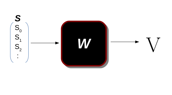
𝑆 is the state vector (feature vector), 𝑊 is the parameter representing the function and 𝑉 is the Value function of state 𝑠, in this function, we map from state to value of that state 𝑉(𝑠)=𝑡 ;𝑡∈𝑅

we can also use VFA to learn 𝑄 function.

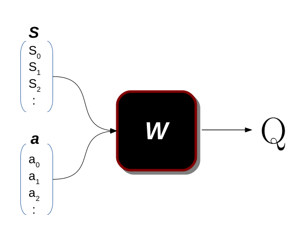
in 𝑄(𝑠,𝑎) we map the pair (𝑠,𝑎) to value. in another world, we say what is the importance of taking action 𝑎 in-state 𝑠.

Benefits of VFA.

• The most important one is Generalization as a human who loves to generalize all problem they face we are seeking to make the computer have that skill. (E.g. if a human sees one or two doors, then they will recognize any types of doors they will see in the future, but for computers, it needs many examples to learn that, but if it can recognizing them then we made a good model). in our case, we want the agent learning to take action in some state even if he did not sea it before.
• Reducing memory, if we use parametrized function instead of the tabular representation we will reduce the memory usage if the state and/or action space is enormous. (E.g. if there is 1∗10⁶ state and 50 action, then I need a table with (50∗10⁶)) entries and that a lot while I can use 10⁴ parameter to approximate this function.
• Reducing computation in most cases, (E.g. if we take the previous example where we need (50∗10⁶) entries ) to solve this problem using 𝑄−𝑙𝑒𝑎𝑟𝑛𝑖𝑛𝑔 algorithm we need for each iteration 𝑂(𝑁²) which is ∼10¹².

Deep Q-learning

after we briefly introduce the VFA we will implement one of the most popular papers in the last 10 years. in this section, we will implement the Deep Q-learning(DQN) algorithm using the OpenAI environment and Tensorflow frameworks. The “Mnih, etc. Playing Atari with Deep Reinforcement Learning 2013”. introduce DQN for the first time. The authors in this paper train an agent to play Atari 2600 games from raw pixels and that was amazing because the agent doesn’t know anything about the environment, or the role of the games even though he can play as human or even better for some games.

I really recommend reading this paper because it’s very simple and easy to understand, and it will make reading future papers easier.

𝑁𝑜𝑡𝑒: please read this section carefully, you should understand every detail because we will reuse the code from this section in future lectures.

#import dependencies library# the environment library
import gym#the AI framework 
import tensorflow as tf
import tensorflow.keras as keras 
import numpy as np#just for ploting stuf
import cv2
import matplotlib.pyplot as plt
import tqdmfrom collections import deque

After we import dependencies we will create our environment using the gym library, we have chosen the breakout game as the playground game.

# make the environment we chose breakout game to try on.
environment=gym.make("Breakout-v4")
state=environment.reset()
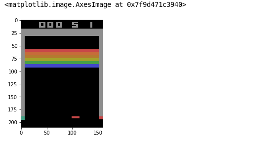
plt.imshow(state)

The First step is to make some prepossessing to each frame, we want to change the RGB format to gray format and that decreases the confusion in the network and we will cut the top of the frame which represent the score which changes and may confuse the training process.

def preprocess_frame(frame):
    image=frame[25:-10,5:-5,:]
    image=tf.image.rgb_to_grayscale(image)
    image=tf.image.resize(image,[84,84])
    image=tf.reshape(image,[85,85])
    image=image/255.0
    return imagedef ploting_function_one(frame):
    image=frame[25:,:,:]
    image=cv2.cvtColor(image,cv2.COLOR_RGB2GRAY)
    image=cv2.resize(image,(85,85))
    return image

This function makes preprocessing steps for each frame from the game.

parameter:

• frame: is a row frame with [210 * 64 * 3] size provided by the environment after we make an action that changes the world, the environment provides us with new observations after applying that action.

return :

• image: processing frame where we cut some of the borders and keep the play area and change the image to grayscale then resize it to [84 , 84] shape and finally normalize pixel value to become in the range [0–1]

The above cell contains two preprocessing functions one for visualization because we can’t plot tensor from TensorFlow

class FireResetEnv(gym.Wrapper):
    def __init__(self, env=None):
        super(FireResetEnv, self).__init__(env)
        assert env.unwrapped.get_action_meanings()[1] == 'FIRE'
        assert len(env.unwrapped.get_action_meanings()) >= 3
        
    def step(self, action):
        return self.env.step(action)
    
    def reset(self):
        self.env.reset()
        obs, _, done, _ = self.env.step(1)
        if done:
            self.env.reset()
            obs, _, done, _ = self.env.step(2)
            if done:
                self.env.reset()
        return obs

This class is Wrapper where we make sure that the game is running, because in some environments in gym library should start the game by action “ 1 “ in most of the game so by doing this we make sure that the game is rolling.

now after we process the frame we need to stack some frames together to represent a one-state so by using that we can give some information about velocity. first lets create a queue with a fixed size 4 so after each move, we push the frame to the queue and then stack them together to represent the 3D block that represents the state. now after we process the frame we need to stack some frames together to represent a one-state so by using that we can give some information about velocity.

stacked_blocks=deque(maxlen=4)def state_creator(frame,is_new_episod,stacked_blocks,number_of_frame=4):
    if is_new_episod:
        image=preprocess_frame(frame)
        for i in range(number_of_frame):
            stacked_blocks.append(image)
    else:
        image=preprocess_frame(frame)
        stacked_blocks.append(image)
    
    state=tf.stack(stacked_blocks,axis=2)
    return state

In this function, we stack the last 4 frames together to perform one state and that gives us some intuition about velocity.

parameter :

• frame: which is the game observation.
• is_new_episod: a boolean parameter that checks if there is no previous frame and that happened at the beginning of each episode.
• stacked_blocks: is deque with max length 4 that save the last 4 frames for us.
• number_of_frame: is by default 4 but we can change it to another number and that makes our state more complex.

return :

• state: tensor with [84,84,4] shape which represents the state of our world.

Now let’s build the model which is a Convolutional Neural Network that contains just 2 layers. the DNN will take a state which is tensor [84,84,4] and the output vector has the same dimension of the action space. This means for each state I will learn how important to take each action in that state in one shot.

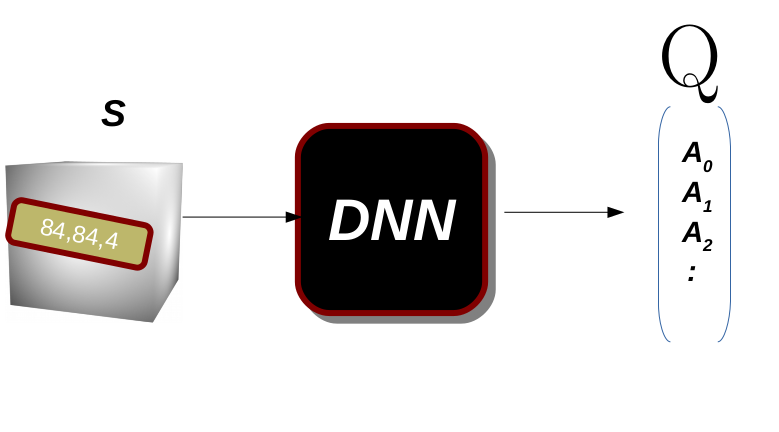
as we can see in the figure the model will learn the importance of all actions for each state, so if we take the action with the highest value then these should lead to the best reward.

#this model is as recomende from paper "Mnih 2013, Playing Atari with Deep Reinforcement Learning"
keras.backend.clear_session()model=keras.Sequential([
    keras.layers.Conv2D(16,8,strides=4,padding='valid',activation='relu',input_shape=[84,84,4]),
    keras.layers.Conv2D(32,4,strides=2,padding='valid',activation='relu'),
    keras.layers.Flatten(),
    keras.layers.Dense(256,activation='relu'),
    keras.layers.Dense(action_space)
])
model.summary()

Instead of training the DQN based only on the latest experiences, we will store all experiences in a replay buffer (or replay memory), and we will sample a random training batch from it at each training iteration. This helps reduce the correlations between the experiences in a training batch, which tremendously helps training.

# this represent the memory where we keep the last million state for training.
replay_buffer=deque(maxlen=1000000)def sample_experiences(batch_size):
    indices=np.random.randint(len(replay_buffer),size=batch_size)
    batch=[replay_buffer[index] for index in indices]
    states,actions,rewords,dones,next_states=[np.array([experiance[field_index] for experiance in batch]) for field_index in range(5)]
    return states,actions,rewords,dones,next_states

This function is use to sample batch from our memory.

parameter :

• batch size: is numeber of example that provided to our network.

return:

• states:it’s tensore [batch_size, image_width, image_height, stacked_size] in our case [32, 84, 84, 4]
• actions: it’s 2D array [batch_size, action] it’s the action in each state in our batch
• rewards: it’s 2D array [batch_size, reward] it’s the reward in each state in out batch
• dones : it’s 2D array [batch_size, done ] where done is boolean value help us to compute the target.
• next_state: it’s tensore [batch_size, image_width, image_height, stacked_size] in our case [32, 84, 84, 4]

𝜖−𝑔𝑟𝑒𝑒𝑑𝑦

Algorithm

we mention before the 𝜖−𝑔𝑟𝑒𝑒𝑑𝑦 in lecture [3] , the pesudocode of the algorithm is as follow and the function epsilon_greedy_policy is just implementation of this algorithm.

• 𝜖←1
• 𝑎←𝑟𝑎𝑛𝑑𝑜𝑚−𝑣𝑎𝑙𝑢𝑒∈[0,1]
• 𝑖𝑓𝑎<𝜖
• take random 𝑎∈𝐴
• 𝑒𝑙𝑠𝑒
• chose the greedy action using the estimator (e.g. 𝑎𝑟𝑔𝑚𝑎𝑥𝑎𝑄(𝑠,𝑎))
• 𝜖←𝑢𝑝𝑑𝑎𝑡𝑒

def epsilon_greedy_policy(state,epsilon):
    if np.random.rand()<epsilon:
        return np.random.randint(action_space)
    else:
        Q_values=model.predict(state[np.newaxis])
        return tf.argmax(Q_values[0])
def play_one_step(env,state,epsilon):
  
    action=epsilon_greedy_policy(state,epsilon)
    next_state,reward,done,info=env.step(action)
    if info['ale.lives']< 5:
            done=True
    stacked_next_state=state_creator(next_state,False,stacked_blocks)
    replay_buffer.append((state,action,reward,done,stacked_next_state))
    return stacked_next_state,reward,done,info

The Play one step function makes action and gets the observation from the world. we make an action and then get the full observation from our environment applying the state_create function to our observation(frame) and then save it in the memory for the training step.

parameter :

• env: it represents our world or environment we work on
• state: it’s the current state.
• epsilon: it’s the threshold we use for action selection

return :

• next_state: tensor [84,84,4] block represent the last 4 frame.
• reward: it’s float number the reward we get after we do some action.
• done: it’s boolean refer if the game finish or not
• info: its dictionary has the counter of lives.

loss_function=tf.losses.mean_squared_error
optimizer=tf.optimizers.Adam(lr=0.00025)

We use the mean squared error as loss function and Adam optimizer the Authors in [1] use RMSprop instead but as Adam is less sensitive to step size then it’s better to use.

in Lecture 3, we introduce the 𝑄−𝑙𝑒𝑎𝑟𝑛𝑖𝑛𝑔 algorithm and in the previous lecture we implement it, lets first back to the algorithm.

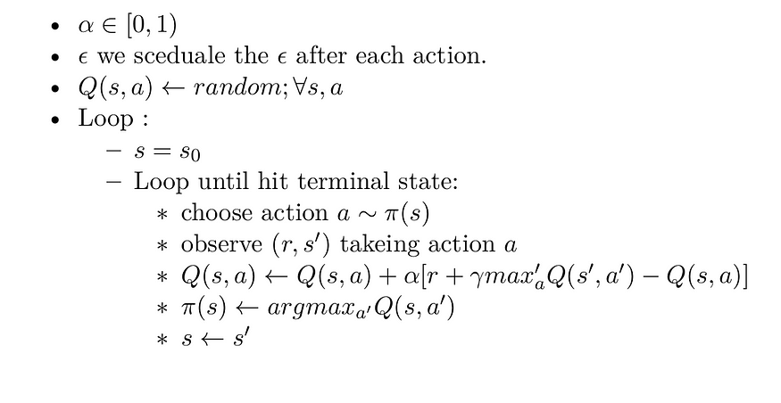
but hear we use function approximation, not tabular representation. so as we say in the first section we will use the return as the target to our model. we mention before the 𝑇𝐷−𝑡𝑎𝑟𝑔𝑒𝑡=𝑅ₜ+𝛾𝑉(𝑠ₜ₊₁) and that what will use hear as target for our model. In a sense, the update 𝑠↦𝑢 means that the the estimated value for state 𝑠 should be more like the update target 𝑢, in another world the model will try to minimize the difference between the value of the current state and the value of the return from the next state and that true because if we are using the optimal action in each state then the value of each state must be close to each other.

def training_step(batch_size,discount_factor):
    #sample experience from the replay buffer
    # states  → s , next states → s' , rewards → r , actions → a. in the algorithm above. 
    states,actions,rewards,dones,next_states=sample_experiences(batch_size)
    
    # max′a Q(s′,a′)
    next_Q_values=model.predict(next_states)
    max_next_Q_values=np.max(next_Q_values,axis=1)
    # [r + gamma * max′a Q(s′,a′)]
    target_Q_values=rewards+(1-dones)*discount_factor*max_next_Q_values
    # this mask will help us reducing the value of the model to just action we made.
    mask = tf.one_hot(actions, action_space)
    # start computing the gradient 
    with tf.GradientTape() as tape:
        # Q(s,a)
        all_Q_values=model(states)
        # this step its to chose only the action we make not all actions for each state. 
        Q_values=tf.reduce_sum(all_Q_values*mask,axis=1,keepdims=True)
        # [r + gamma * max′a Q(s′,a′)] - Q(s,a) 
        loss=tf.reduce_mean(loss_function(target_Q_values,Q_values))
    # compute the gradient for model variables
    gradiants=tape.gradient(loss,model.trainable_variables)
    # make the optimization step.
    optimizer.apply_gradients(zip(gradiants,model.trainable_variables))

This function is responsible for doing one training step where we sample one batch from the replay buffer then we push this batch in our model for the forward step and apply gradient with optimizer by hand.

parameter :

• batch_size: the number of training examples we sample
• discout_factor: this parameter is responsible for future rewards important its value must be in the range[0–1]

return:

• None, where it’s applying the change in place for model parameter.

The last step is creating the training loop, we will use the function we created above.

episodes=700
epsilon=1.0
batch_size=5
discount_factor=0.98for episode in tqdm.tqdm(range(episodes)):
    state=environment.reset()
    stacked_state=state_creator(state,True,stacked_blocks)
    rewards=0
    epsilon=max(1-episode/500,0.1)
    while True:
        stacked_state,reward,done=play_one_step(environment,stacked_state,epsilon)
        rewards+=reward
        if done:
            if not (episode%10) :
                print(rewards)
            break
            
        if len(replay_buffer)>50:
            training_step(batch_size,discount_factor)

Now let’s put it all together in one class, you can check the full code in Github.

I create the DQN_Agent class which will encapsulate all the functions above and I provide it with default parameters as in the paper we implemented.

𝑁𝑜𝑡𝑒: in the next lectures, we will just edit this class, I will refer to the editing line by ⟶ sign.

Summary:

in this lecture we introduce Function Approximation which is a very powerful concept in Machine learning, and AI field in General we also implement the Deep 𝑄−𝑙𝑒𝑎𝑟𝑛𝑖𝑛𝑔 algorithm to play breakout game.

I hope you find this article useful and I am very sorry If there is any error or Misspelled in the article, Please do not hesitate to contact me, or drop comment to correct things.

Khalil Hennara
Ai Engineer at MISRAJ