in this lecture, we will implement 3 papers,[2] Mnih,etc. Human-level control through deep reinforcement learning ,[3] Hasselt,etc. Deep Reinforcement Learning with Double Q-learning and [4] Wang,etc. Dueling Network Architectures for Deep Reinforcement Learning.

but before that, we will back to the last lecture where we introduce function approximation and Deep Q-learning. we also implement [1] Mnih,etc. Playing Atari with Deep Reinforcement Learning 2013.in this lecture we will improve the DQN algorithm to achieve better performance.

Fixed DQN

The First alternative to the DQN is called Fixed-DQN from [2] Mnih, etc. Human-level control through deep reinforcement learning paper, in this paper the authors introduce a little modification to the previous paper [1]. Because Reinforcement learning is known to be unstable or even to diverge when a nonlinear function approximator such as a neural network is used to represent the action-value (also known as Q) function. This instability has several causes:

• The correlations present in the sequence of observations, the fact that small updates to Q may significantly change the policy and therefore change the data distribution
• The correlations between the action-values (Q) and the target values 𝑟+𝛾𝑚𝑎𝑥ₐ′𝑄(𝑠′,𝑎′)

For the first problem, we solve it in the previous lecture using replay buffer that randomizes over the data, thereby removing correlations in the observation sequence and smoothing over changes in the data distribution

For the second one, we used an iterative update that adjusts the action-values (Q) towards target values that are only periodically updated, thereby reducing correlations with the target. instead of using one model to predict the Target and the Q-value for the current state the author makes two models (Deep neural networks) with identical structures. and use one for predicting the Target and the other for learning the Q_value.

in the previous lecture, the loss function for 𝑄−𝑙𝑒𝑎𝑟𝑛𝑖𝑛𝑔 function is:

𝐿(𝜃ᵢ)=𝐸[(𝑟+𝛾𝑚𝑎𝑥ₐ′𝑄(𝑠ₙₑₓₜ,𝑎′,𝜃ᵢ)−𝑄(𝑠,𝑎,𝜃ᵢ))²]

where the 𝑟+𝛾𝑚𝑎𝑥ₐ′𝑄(𝑠𝑛𝑒𝑥𝑡,𝑎′,𝜃ᵢ) is the target and 𝜃ᵢ is the parameter of the model and the Expectation is just taking the average loss over one batch training. as we can notice in equation (1) the model that predicts the target and the Q-value is the same. we will use two models instead of one, and then update the target model for each 𝐾 step.

Does this Idea help in reducing noise?

Answer:

any supervised learning problem consist of pairs [(𝑥1,𝑦1),(𝑥2,𝑦2),…(𝑥𝑛,𝑦𝑛)]∼𝐷

where each pair is a training example from the distribution 𝐷 we want to estimate. if 𝑦 is fixed, then if we train a good estimator (depends on the data, problem, desired solution, etc ) we will converge to the True distribution or we will be very close to it. The RL problem is the label 𝑦, it’s changing over time, so if we use the previous concept, the target 𝑦 will stay fixed for (k step), which makes the training more stable and efficient than before.

The notation for the new algorithm: 𝑄(𝑠,𝑎,𝜃ᵢ⁻) is used for predict the target while 𝑄(𝑠,𝑎,𝜃ᵢ⁺) is used for learn the 𝑄−𝑣𝑎𝑙𝑢𝑒

function.we will called the first model the Target model and the second one online model.

The loss function becomes:

𝐿(𝜃ᵢ⁺)=𝐸[(𝑟+𝛾𝑚𝑎𝑥ₐ′𝑄(𝑠ₙₑₓₜ,𝑎′,𝜃ᵢ⁻)−𝑄(𝑠,𝑎,𝜃ᵢ⁺))²]

and each 𝑘 step we update the target model using the online model, 𝑄(𝜃⁻)←𝑄(𝜃⁺) we set the target model parameters equal to the online model parameter each 𝑘 step:

Now we will update the code from the previous lecture.

𝑁𝑜𝑡𝑒:

we will just edit the DQN_Agent class, I will refer to the editing line by ⟶sign.

you can use the full code hear.

#this model is as recomende from paper "Mnih et al., 2015; van Hasselt et al., 2015"
keras.backend.clear_session()model=keras.Sequential([
    keras.layers.Conv2D(32,8,strides=4,padding='valid',activation='relu',input_shape=[84,84,4]),
    keras.layers.Conv2D(64,4,strides=2,padding='valid',activation='relu'),
    keras.layers.Conv2D(64,3,strides=1,padding='valid',activation='relu'),
    keras.layers.Flatten(),
    keras.layers.Dense(512,activation='relu'),
    keras.layers.Dense(action_space)
])
model.summary()

The first change is the model structure is a small change but makes a difference.

class Fixed_DQN_Agent:
    self.online_model=model
    self.target_model=keras.models.clone(model)
    self.target_model.set_weights(model.get_weights())

the second change, we have 2 models instead of one model, the online_model and target_model the first one it’s used for computing the 𝑄−𝑣𝑎𝑙𝑢𝑒 function at each time step while the other just computes the target. the target model has the same structure as the online model and the same initial parameter.

self.update_rate=update_steps

Another update to the previous algorithm, where we need a parameter that defines the update rate for the target model.

def _epsilon_greedy_policy(self,state,epsilon):
        if np.random.rand()<epsilon:
            return np.random.randint(self.action_space)
        else:
#---->      hear we use the online model for prediction of best action.
            Q_values=self.online_model.predict(state[np.newaxis])
            return tf.argmax(Q_values[0])

Because we have two models now, we need to use the online model in the 𝜖−𝑔𝑟𝑒𝑒𝑑𝑦 policy because it’s the model that estimates the 𝑄−𝑣𝑎𝑙𝑢𝑒 function.

def _training_step(self):
    # get the batch from the replay_buffer (our memory)
    states,actions,rewards,dones,next_states=self._sample_experiences()
#---->  the online_Q(state,a)=online_Q(state,a) + alpha [ reward + gamma * max (target_Q(next_state,a) for all a) - online_Q(state,a)] 
    next_Q_values=self.target_model.predict(next_states)
    max_next_Q_values=np.max(next_Q_values,axis=1)
    # compute the target which is [reward +  gamma * max(target_Q(next_state,a) over a)] 
    target_Q_values=rewards+(1-dones)*self.discount_factor*max_next_Q_values#this mask it's important for vanishing the value of actions that we don't used it's 2D array with 1 if action i was picked and zero othewise.
    mask = tf.one_hot(actions, self.action_space)#start the gradient recording to compute the gradient for our model.
    with tf.GradientTape() as tape:
#---->      compute the Q function for current state (hear for the whole batch).
        all_Q_values=self.online_model(states)
        #hear we use the mask so we reduce the result for just the action we picked.
        Q_values=tf.reduce_sum(all_Q_values*mask,axis=1,keepdims=True)
        #computer the loss function with the target we compute erlaier.
        loss=tf.reduce_mean(self.loss_function(target_Q_values,Q_values))
#---->      compute the gradient for our  online_model parameter.
    gradiants=tape.gradient(loss,self.online_model.trainable_variables)
#---->  apply the optimization step using the gradient we compute for the online_model
    self.optimizer.apply_gradients(zip(gradiants,self.online_model.trainable_variables))

The training_step function also has some changes, now the target model predicts the target. while when we made the optimization step we update the parameter of the online model.

def fit(self):
    # 
    # all line are the same 
    #-----> hear where update the target model after 100 episod by set the parameter as online model.
    if episode%self.update_rate:
        self.target_model.set_weights(self.online_model.get_weights())

the last update is in the fit function where we update the target model after 𝑘 steps by setting its parameters as the online model

Double Q-learning

is almost the Fixed-Q-learning but with a little change in who to predict the target. It is an open question whether, if the overestimation do occur, this negatively affects performance in practice. Overoptimistic value estimates are not necessarily a problem in and of themselves. If all values would be uniformly higher then the relative action preferences are preserved and we would not expect the resulting policy to be any worse. Furthermore, it is known that sometimes it is good to be optimistic. optimism in the face of uncertainty is a well-known exploration technique Kaelbling et al., 1996. If, however, the overestimation are not uniform and not concentrated at states about which we wish to learn more, then they might negatively affect the quality of the resulting policy. Thrun and Schwartz, 1993 give specific examples in which this leads to suboptimal policies, even asymptotically. because of Maximization Bias when we use the Fixed-DQN we get bias estimator because of the maximization selection. According to Sun and Tsitsiklis, 2007 even if the estimator is unbiased, taking the max over action lead to bias policy.

E.g.: Consider single-state 𝑀𝐷𝑃(|𝑆|=1) and there is two action (𝑎₁,𝑎₂), and both action have 0 mean rewards. [𝔼(𝑟|𝑎=𝑎₁)=𝔼(𝑟|𝑎=𝑎₂)=0]. Then 𝑄(𝑠,𝑎₁)=𝑄(𝑠,𝑎₂)=0=𝑉(𝑠) let estimate 𝑄̂ (𝑠,𝑎₁),𝑄̂ (𝑠,𝑎₂). Use unbiased estimator for 𝑄:e.g. 𝑄̂ =(1/𝑛) ∑ᵢ 𝑟ᵢ(𝑠,𝑎₁) where 𝑛 is the number of taking action 𝑎₁. let 𝜋̂ =𝑎𝑟𝑔𝑚𝑎𝑥ₐ𝑄̂ (𝑠,𝑎₁) be the greedy policy Even though each estimate of the state-action values is unbiased, the estimate of 𝜋̂ 𝑣𝑎𝑙𝑢𝑒𝑉̂ 𝜋 is biased.

𝑝𝑟𝑜𝑜𝑓:

𝑉̂ =𝔼[𝑚𝑎𝑥(𝑄(𝑎₁),𝑄(𝑎₂))]

≥𝑚𝑎𝑥𝔼[𝑄(𝑎₁),𝑄(𝑎₂)]

=𝑚𝑎𝑥[0,0]

=0

=𝑉𝜋

We can notice in the second line, the estimated value is ≥ than the True value.

The idea behind the Double Q-learning algorithm van Hasselt, 2010, which was first proposed in a tabular setting, gives a solution to this problem called Double Q-learning. The Idea is as follows, split the samples and use them to create two independent unbiased estimates of 𝑄₁(𝑠,𝑎ᵢ),𝑄₂(𝑠,𝑎ᵢ);∀𝑎

• use one estimate to select max action 𝑎*=𝑎𝑟𝑔𝑚𝑎𝑥ₐ𝑄₁(𝑠,𝑎)
• use other estimate to estimate value of 𝑎*:𝑄₂(𝑠,𝑎*)
• yields unbiased estimate: 𝔼(𝑄₂(𝑠,𝑎*))=𝑄₂(𝑠,𝑎*)

This Idea can be generalized to work with arbitrary function approximation, including deep neural networks.

In the previous section, we introduce the Fixed_DQN and show that the Target follows equation (2), as stated by [3], we will predict the target using the following equation.

𝑌ᴰᵒᵘᵇˡᵉ=𝑅ₜ₊₁+𝛾𝑄(𝑠ₙₑₓₜ,𝑎𝑟𝑔𝑚𝑎𝑥ₐ𝑄(𝑠ₙₑₓₜ,𝑎,𝜃⁺),𝜃⁻)

where 𝑄(;𝜃⁻) is target model and 𝑄(;𝜃⁺)

is the online model.

Notice that the selection of the action, in the argmax, is still due to the online weights 𝜃⁺.

as in the Q-learning, we are still estimating the value of the greedy policy according to the current values, as defined by 𝜃⁺. However, we use the second set of weights 𝜃⁻ to fairly evaluate the value of this policy. This second set of weights can be updated as in the previous section (each 𝑘 step).

we will update the Fixed_DQN Agent you can get the full code.

def _training_step(self):
    # get the batch from the replay_buffer (our memory)
    states,actions,rewards,dones,next_states=self._sample_experiences()
#---->  the online_Q(state,a)=online_Q(state,a) + alpha [ reward + gamma * target_Q(next_state,argmax online_Q(next_state,a_i) for all a)-online_Q(state,a)] 
#---->  as we can see hear we replace the prediction from the target model to online model as "Hado van Hasselt 2015" recomend 
    next_Q_values=self.online_model(next_states)
#---->  hear we take the best action over all action for the whole batch     
    best_action=np.argmax(next_Q_values,axis=1)
#---->  create mask for reducing the value of actions that we don't used.        
    best_action_mask = tf.one_hot(best_action, self.action_space).numpy()#---->  compute the target which is [reward +  gamma * target_Q(next_state,argmx online_Q(next_state,a) over a) ]    
    max_next_Q_values=(self.target_model(next_states) * next_mask).sum(axis=1)
    target_Q_values=rewards+(1-dones) * self.discount_factor * max_next_Q_values
    #
    #The rest is the same as before

Dueling DDQN

The only difference in Dueling-DDQN is the model structure not the algorithm in the paper Ziyu Wang etc.. 2016 show that a little change in the model structure outperforms the old algorithm so instead we predict the 𝑄(𝑠,𝑎)

directly we first predict the 𝑉(𝑠) and 𝐴(𝑠,𝑎) where 𝐴(𝑠,𝑎) is the advantage as describe in Birds 1993

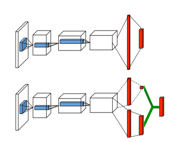
where, 𝐴(𝑠,𝑎) =𝑄(𝑠,𝑎)-𝑉(𝑠) where the value function 𝑉 measures the how good it is to be in a particular state 𝑠. The 𝑄 function, however, measures the value of choosing a particular action when in this state. The advantage function 𝐴 subtracts the value of the state from the Q function to obtain a relative measure of the importance of each action. we design a single Q-network architecture, as illustrated in Figure 1, which we refer to as the dueling network. The lower layers of the dueling network are convolutional as in the original DQNs (Mnih et al., 2015). However, instead of following the convolutional layers with a single sequence of fully connected layers, we instead use two sequences (or streams) of fully connected layers. The streams are constructed such that they have the capability of providing separate estimates of the value and advantage functions. Finally, the two streams are combined to produce a single output Q.

𝑄(𝑠,𝑎) = 𝑉(𝑠) + 𝐴(𝑠,𝑎)

𝑉(𝑠) is scaler output so the stream output for this branch has 1 output neuron while 𝐴(𝑠,𝑎) has as many as available actions we have so the output of this stream has |𝐴𝑐𝑡𝑖𝑜𝑛𝑠| neuron.

However, we need to keep in mind that 𝑄(𝑠,𝑎) is only a parameterized estimate of the true Q-function. Moreover, it would be wrong to conclude that 𝑉(𝑠) is a good estimator of the state-value function, or likewise that 𝐴(𝑠,𝑎) provides a reasonable estimate of the advantage function

The equation above is unidentifiable in the sense that given 𝑄 we cannot recover 𝑉 and 𝐴 uniquely. To see this, add a constant to 𝑉(𝑠) and subtract the same constant from 𝐴(𝑠,𝑎). This constant cancels out resulting in the same 𝑄 value. This lack of identifiability is mirrored by poor practical performance when this equation is used directly. To address this issue of identifiability, we can force the ad- vantage function estimator to have zero advantage at the chosen action. That is, we let the last module of the net- work implement the forward mapping

𝑄(𝑠,𝑎) = 𝑉(𝑠) + ( 𝐴(𝑠,𝑎) − max ₐ𝐴(𝑠,𝑎))

Now, for 𝑎* = 𝑎𝑟𝑔𝑚𝑎𝑥ₐ 𝑄(𝑠,𝑎) = 𝑎𝑟𝑔𝑚𝑎𝑥ₐ 𝐴(𝑠,𝑎)

we obtain 𝑄(𝑠,𝑎*)=𝑉(𝑠). Hence, the stream 𝑉(𝑠) provides an estimate of the value function, while the other stream produces an estimate of the advantage function. An alternative module replaces the max operator with an average:

𝑄(𝑠,𝑎)=𝑉(𝑠)+[𝐴(𝑠,𝑎)−(1/|𝐴|)∑ₐ 𝐴(𝑠,𝑎)]

On the one hand, this loses the original semantics of 𝑉 and 𝐴

because they are now off-target by a constant, but on the other hand it increases the stability of the optimization: with last equation, the advantages only need to change as fast as the mean, instead of having to compensate any change to the optimal action’s advantage, so we will implement the last equation to our model.

The model architecture is the same as shown in Mnih etc. 2015, Hasselt, etc. 2015 but with to stream of a fully connected layer.

#this model is as recomende from paper "Ziyu Wang et al., 2016 "
# to build the model we will use the Functinal API of keras.
keras.backend.clear_session()inputs = keras.layers.Input(shape=[84,84,4])
x=keras.layers.Conv2D(32,8,strides=4,padding='valid',activation='relu')(inputs)
x=keras.layers.Conv2D(64,4,strides=2,padding='valid',activation='relu')(x)
x=keras.layers.Conv2D(64,3,strides=1,padding='valid',activation='relu')(x)  
x=keras.layers.Flatten()(x)V_h1=keras.layers.Dense(512,activation='relu')(x)
A_h1=keras.layers.Dense(512,activation='relu')(x)state_value=keras.layers.Dense(1)(V_h1)raw_advantage=keras.layers.Dense(action_space)(A_h1)advantage = raw_advantage-tf.reduce_mean(raw_advantage,axis=1,keepdims=True)Q_value= tf.add(advantage , state_value)model=keras.Model(inputs=[inputs],outputs=[Q_value])model.summary()

Then use the previous DDQN_Agent with no change at all, you can get the full code from Github